Hierarchical Data in SQL: The Ultimate Guide

Storing hierarchical data in a database is something we need to do occasionally.

While databases are very good at storing data about different types of records, hierarchical data is not something that is immediately obvious.

But there are several ways it can be done.

In this guide, you’ll learn what hierarchical data is, see several different methods for designing your tables along with queries for each method, pros and cons of each design, and recommendations for Oracle, SQL Server, MySQL, and PostgreSQL.

Let’s get into the guide!

What is Hierarchical Data?

You might have heard the term “hierarchical data” or “hierarchical queries” before but may not know exactly what it means.

Or the term may be completely new to you.

So, what is hierarchical data?

It’s a data structure where records are parents or children of other records of the same type. A common example is employees and managers: employees and managers are both employees of a company. A manager can have employees they manage, and can also have a manager themselves.

Another example of hierarchical data is product categories.

Say you’ve got a database for an eCommerce website. You have products and each of those are in categories. Your categories could be high-level categories such as Clothing, Toys, and Homewares.

But you may also have subcategories within those: in Clothing you may have Pants, Jackets, Shoes. And within those subcategories you may have even more categories.

 

Why does it need a specific design?

Employees and product categories are two examples of hierarchical data, and there are many more.

But why does hierarchical data need to be considered? Why does the design need to be thought about specifically? Can’t we just add it to tables like normal?

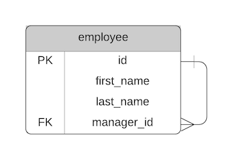
Let’s try and do that for our employee example.

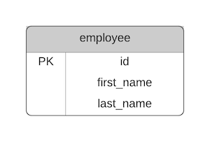
Say we have an employee table that stores information about employee: an ID, first name, last name:

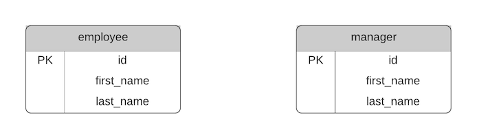
We also want to store managers. So let’s create a new table for manager, which also has an ID, first name, and last name.

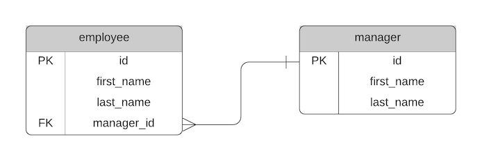
We want to see which manager is the manager of each employee, so we add a manager_id foreign key to the employee table.

Makes sense so far, right?

But then, what if the manager also has a manager? For example, a Team Member > Team Leader > Area Manager.

We could add a new table called area_manager to represent these more senior managers. It would also have an ID, first name, and last name. We would also add an area_manager_id into the manager table.

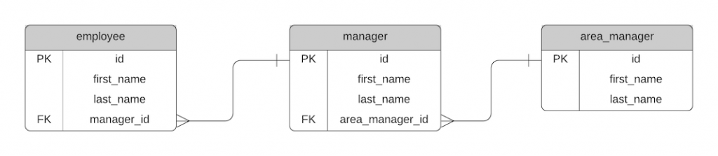
We now have three tables here, which capture this relationship.

However, there are several problems with this:

• All of the tables are similar, storing the same kind of information. This is a kind of duplication.
• Employee structures need to follow this pattern. An area manager cannot have employees directly if we use this design.
• If an employee changes roles, we need to move them to a new table.
• If we have additional levels of management, we need new tables. This could mean we have 4, 5, 6 or more tables to record employee hierarchy.

So what’s the solution?

There are many ways to implement a design that solves this, but the concept essentially looks like this:

This demonstrates a single table or single type of record. It has a join to itself, called a self join, that shows one record can be related to another record of the same type.

Employees are related to other employees as a manager.

Product categories are parent categories of other categories.

The specifics of how this is done is shown below. There are several ways to do this, each of which have their pros and cons.

For each of these examples, we’ll try to capture the following employee hierarchy:

• Claire
  • Steve
    • Nathan
    • Paula
  • Sarah
    • Anne
    • Roger
    • Tim
    • Peter
  • John
    • Hugo
      • Matthew
      • Ruth
      • Simon

The head of the company is Claire, who has Steve, Sarah, and John as direct reports. Working in each of those teams are several other team members.

Let’s take a look at how you can design database tables to handle hierarchical data.

While we’re here, if you want an easy-to-use PDF guide for the main features in different database vendors, get my SQL Cheat Sheets here:

 

Adjacency List

Adjacency List is a design method for implementing hierarchical data. It’s achieved by storing the ID of the related record on the desired record. You add one column to your table, and set it as a foreign key to the same table’s primary key.

This is the method that I recommend using for most cases.

I’ll explain more in the pros and cons for each design, and in the summary at the end of the guide.

Here’s what the ERD looks like:

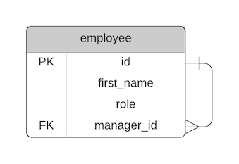
So, let’s say you have a table of employees like this:

id	first_name	role
1	Claire	CEO
2	Steve	Head of Sales
3	Sarah	Head of Support
4	John	Head of IT
5	Nathan	Salesperson
6	Paula	Salesperson
7	Anne	Customer Support Officer
8	Roger	Customer Support Officer
9	Tim	Customer Support Officer
10	Peter	Assistant
11	Hugo	Team Leader
12	Matthew	Developer
13	Ruth	Developer
14	Simon	QA Engineer

To implement an Adjacency List design, you would add a new column called manager_id (or something similar). This new column would refer to the id in the same table: the employee table

id	first_name	role	manager_id
1	Claire	CEO	null
2	Steve	Head of Sales	1
3	Sarah	Head of Support	1
4	John	Head of IT	1
5	Nathan	Salesperson	2
6	Paula	Salesperson	2
7	Anne	Customer Support Officer	3
8	Roger	Customer Support Officer	3
9	Tim	Customer Support Officer	3
10	Peter	Assistant	3
11	Hugo	Team Leader	4
12	Matthew	Developer	11
13	Ruth	Developer	11
14	Simon	QA Engineer	11

The CEO has a manager_id of NULL, as they don’t have a manager. All other employees have a manager_id.

For example, Steve, the Head of Sales, has a manager_id value of 1. This refers to employee ID 1, which is Claire.

Ruth, employee ID 13, has a manager_id of 11, which is Hugo, a Team Leader.

It’s the most common example of achieving hierarchical data in a relational database.

 

Select Employee and their Manager

We can select an employee and their manager by using a LEFT JOIN on the same table. We use a LEFT JOIN to include employees without managers.

SELECT e.id, e.first_name, e.role, e.manager_id, m.first_name
FROM employee e
LEFT JOIN employee m ON e.manager_id = m.id;

The results are:

id	first_name	role	manager_id	first_name
1	Claire	CEO	null	null
2	Steve	Head of Sales	1	Claire
3	Sarah	Head of Support	1	Claire
4	John	Head of IT	1	Claire
5	Nathan	Salesperson	2	Steve
6	Paula	Salesperson	2	Steve
7	Anne	Customer Support Officer	3	Sarah
8	Roger	Customer Support Officer	3	Sarah
9	Tim	Customer Support Officer	3	Sarah
10	Peter	Assistant	3	Sarah
11	Hugo	Team Leader	4	John
12	Matthew	Developer	11	Hugo
13	Ruth	Developer	11	Hugo
14	Simon	QA Engineer	11	Hugo

This shows the employee ID, name, and role. It also shows their manager’s employee ID and first name.

 

Selecting the Tree

If this is the database design, how can we select all of the records in the hierarchy?

Our query would look like this:

WITH subquery_name AS (
  anchor_query
  UNION ALL
  recursive_query
)
SELECT cols
FROM subquery_name;

This query works by using a WITH clause which contains an anchor query (selecting the root node, or the employee with no manager) and the recursive query (selecting all of the remaining employees).

This will result in a list of all employees with their level from the top level, or root node.

The actual query looks like this:

SQL Server

WITH empdata AS (
  (SELECT id, first_name, role, manager_id, 1 AS level
  FROM emp_h
  WHERE id = 1)
  UNION ALL
  (SELECT this.id, this.first_name, this.role, this.manager_id, prior.level + 1
  FROM empdata prior
  INNER JOIN emp_h this ON this.manager_id = prior.id)
)
SELECT e.id, e.first_name, e.role, e.manager_id, e.level
FROM empdata e
ORDER BY e.level;

The results are:

id	first_name	role	manager_id	first_name	level
1	Claire	CEO	null	Claire	1
2	Steve	Head of Sales	1	Steve	2
3	Sarah	Head of Support	1	Sarah	2
4	John	Head of IT	1	John	2
5	Nathan	Salesperson	2	Nathan	3
6	Paula	Salesperson	2	Paula	3
7	Anne	Customer Support Officer	3	Anne	3
8	Roger	Customer Support Officer	3	Roger	3
9	Tim	Customer Support Officer	3	Tim	3
10	Peter	Assistant	3	Peter	3
11	Hugo	Team Leader	4	Hugo	3
12	Matthew	Developer	11	Matthew	4
13	Ruth	Developer	11	Ruth	4
14	Simon	QA Engineer	11	Simon	4

This query works in SQL Server. In MySQL and PostgreSQL, we need to add the word RECURSIVE after the WITH keyword. This will work in MySQL 8.0 when the WITH clause was introduced, but not in earlier versions.

You can also use the HierarchyID data type in SQL Server when working with hierarchies. More information on this is available here.

MySQL and PostgreSQL

WITH RECURSIVE empdata AS (
  (SELECT id, first_name, role, manager_id, 1 AS level
  FROM employee
  WHERE id = 1)
  UNION ALL
  (SELECT this.id, this.first_name, this.role, this.manager_id, prior.level + 1
  FROM empdata prior
  INNER JOIN employee this ON this.manager_id = prior.id)
)
SELECT e.id, e.first_name, e.role, e.manager_id, e.level
FROM empdata e
ORDER BY e.level;

In Oracle, you can use specific syntax for hierarchical queries. The WITH clause syntax should still work, but this version is Oracle-specific and may be simpler to understand.

Oracle

SELECT id, first_name, role, manager_id, level
FROM employee
START WITH id = 1
CONNECT BY PRIOR id = manager_id
ORDER BY level ASC;

This query will show the same results as above.

The START WITH keyword indicates the top of the tree. In this case it’s the employee with no manager, which has an ID of 1.

The CONNECT BY keyword indicates how the records are related to their parents. PRIOR id means the id of the previous record, and it is equal to the manager_id of this record. It’s the syntax that allows for the hierarchy to be queried.

 

Select Part of the Tree

To select part of the tree, such as all employees in a department, we simply change the WHERE clause (or START WITH clause in Oracle) to refer to the new ID.

So, to see all employees in IT, we write this query:

WITH empdata AS (
  (SELECT id, first_name, role, manager_id, 1 AS level
  FROM employee
  WHERE id = 4)
  UNION ALL
  (SELECT this.id, this.first_name, this.role, this.manager_id, prior.level + 1
  FROM empdata prior
  INNER JOIN employee this ON this.manager_id = prior.id)
)
SELECT e.id, e.first_name, e.role, e.manager_id, e.level
FROM empdata e
ORDER BY e.level;

The only change is the WHERE id = 4. This means the row with the ID of 4 is now the root node. This record and all records under it are shown.

 

Adding Records

How do we add records to this table?

For example, we may have a new employee join. We can add a record pretty easily. We just need to write an INSERT statement.

Here’s our table:

id	first_name	role	manager_id
1	Claire	CEO	null
2	Steve	Head of Sales	1
3	Sarah	Head of Support	1
4	John	Head of IT	1
5	Nathan	Salesperson	2
6	Paula	Salesperson	2
7	Anne	Customer Support Officer	3
8	Roger	Customer Support Officer	3
9	Tim	Customer Support Officer	3
10	Peter	Assistant	3
11	Hugo	Team Leader	4
12	Matthew	Developer	11
13	Ruth	Developer	11
14	Simon	QA Engineer	11

Let’s say we have a new employee with the following values:

• id: 15
• First Name: Alex
• Role: Salesperson
• Manager: Steve (id 2)

Our INSERT statement would look like this:

INSERT INTO employee (id, first_name, role, manager_id)
VALUES (15, 'Alex', 'Salesperson', 2);

The value is then inserted.

We can run the same SELECT query above to view the data in a hierarchy.

So, inserting a new record is pretty easy. We don’t need to make any updates to any existing records.

 

Moving Records

What happens if an employee changes manager?

We can write an UPDATE statement which changes the manager_id of that employee. They will then appear in the right place in a hierarchical query.

For example, if the employee Peter (id 10) moves from Support to Sales, we can update the manager ID from 3 to 2.

UPDATE employee
SET manager_id = 2
WHERE id = 10;

This will move Peter from Support to Sales. There’s no need to update any other values.

 

Deleting Records

To delete a record, you can write a DELETE statement to remove the record.

DELETE FROM employee WHERE id = 10;

However, if the employee is a manager of other employees, you’ll need to move those employees to a different manager. If you try to delete the records, and a foreign key constraint exists, you’ll get an error.

You can use an UPDATE statement to update the employees of the manager you want to delete, then delete the manager.

 

Pros

The Adjacency List concept has some pros and cons.

Here are the pros:

• It’s easy to implement. It just involves adding a new column that refers to the ID of the parent record in the same table.
• It’s easy to add new items.
• It’s easy to move items to a different place in the hierarchy.
• It’s fairly easy to remove items.

 

Cons

Here are the cons or disadvantages of Adjacency List:

• The query to fetch data is complicated. In most databases you need to write a WITH clause with two queries inside it.
• The query to fetch the entire tree, or subset of the tree, can be slow to run with a large amount of records.
• It can be hard to find the path of a record from the root to the current record.
• Deleting items that have children causes the children’s relationship to break, or the delete will fail, depending on the constraint settings. You’ll need to update the children to move them to a new parent before deleting.

 

A Note on SQL Antipatterns Book

If you’ve read the SQL Antipatterns book by Bill Karwin, you might remember that one of the antipatterns is using the Adjacency List model. The book mentions it seems easy but has problems with querying data.

(If you haven’t read the book, I highly recommend it!)

This book was written quite a while ago, where Oracle 11g and MySQL 5 were the latest versions. The SQL that these (and other) databases support has evolved, and the drawbacks of Adjacency List in the book have mostly been addressed.

 

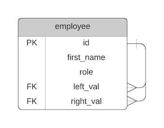
Nested Set

The Nested Set model of hierarchical data is a design that stores the minimum and maximum ID values of the record and all records within it. It’s a good alternative for hierarchical data to Adjacency List.

What does this mean, and how does it work?

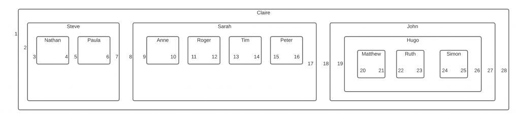
Let’s use our employee example from earlier. Here’s what it looks like as a tree:

• Claire
  • Steve
    • Nathan
    • Paula
  • Sarah
    • Anne
    • Roger
    • Tim
    • Peter
  • John
    • Hugo
      • Matthew
      • Ruth
      • Simon

To understand Nested Sets, it helps to visualise this structure as a series of containers. Each container represents an employee, and within the container are all employees that are managed by this employee.

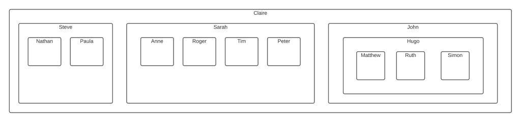
To prepare this for a Nested Sets model, we need to number the left and right edges of each container. This will let us query and maintain the data in the table.

We start with number 1, which is the left border of the largest container. We then add a number 2 to the next border, whether it’s a left or a right border. We keep going until all left and right borders are numbered.

What do we do with these numbers?

You’ll notice that each container has a number on the left and a number on the right. We store these two numbers on the record in the table.

So, we add two numbers to our table: one to store the left number, and one to store the right number.

I’ve called them left_val and right_val, because the words LEFT and RIGHT are built-in functions and using those names as column names could be confusing.

Our table looks like this:

So we’ve made some diagram to number the borders of our records, we’ve added columns to our table, and added these numbers to the table.

What’s the point of this?

It allows us to query the data very easily and very efficiently.

Unlike the Adjacency List method, the Nested Sets method is much easier to query and usually much faster.

Let’s see some examples.

 

Selecting the Tree

To select all of the records in the tree, including their level, our query would look like this:

SELECT e2.id, e2.first_name, e2.role, e2.left_val, e2.right_val
FROM employee e1
INNER JOIN employee e2 ON e2.left_val BETWEEN e1.left_val AND e1.right_val
WHERE e1.id = 1;

This query will find all employees where the left value is between the left and right value of the specified employee ID. In this case, we have specified employee ID 1.

The results are:

id	first_name	role	left_val	right_val
1	Claire	CEO	1	28
2	Steve	Head of Sales	2	7
3	Sarah	Head of Support	8	17
4	John	Head of IT	18	27
5	Nathan	Salesperson	3	4
6	Paula	Salesperson	5	6
7	Anne	Customer Support Officer	9	10
8	Roger	Customer Support Officer	11	12
9	Tim	Customer Support Officer	13	14
10	Peter	Assistant	15	16
11	Hugo	Team Leader	19	26
12	Matthew	Developer	20	21
13	Ruth	Developer	22	23
14	Simon	QA Engineer	24	25

We can see all employees in the table here.

This query will work in all vendors of SQL. It only uses joins, no proprietary syntax, so it’s easier to write than the Adjacency List version.

 

Select Part of the Tree

If we want to see all employees under a specific manager, or just part of the overall hierarchy, we simply change the WHERE clause to start with the ID we want for the root node (or the top level).

So, to see all employees in IT, we write this query:

SELECT e2.id, e2.first_name, e2.role, e2.left_val, e2.right_val
FROM employee e1
INNER JOIN employee e2 ON e2.left_val BETWEEN e1.left_val AND e1.right_val
WHERE e1.id = 4;

This will show the following results:

id	first_name	role	left_val	right_val
4	John	Head of IT	18	27
11	Hugo	Team Leader	19	26
12	Matthew	Developer	20	21
13	Ruth	Developer	22	23
14	Simon	QA Engineer	24	25

The query is almost the same as querying the whole tree.

 

Adding Records

Inserting a new record in the tree is a bit more complex than in the Adjacency List design, because you need to recalculate all of the left and right values greater than the left value of the new record.

For example, here’s our table:

id	first_name	role	left_val	right_val
1	Claire	CEO	1	28
2	Steve	Head of Sales	2	7
3	Sarah	Head of Support	8	17
4	John	Head of IT	18	27
5	Nathan	Salesperson	3	4
6	Paula	Salesperson	5	6
7	Anne	Customer Support Officer	9	10
8	Roger	Customer Support Officer	11	12
9	Tim	Customer Support Officer	13	14
10	Peter	Assistant	15	16
11	Hugo	Team Leader	19	26
12	Matthew	Developer	20	21
13	Ruth	Developer	22	23
14	Simon	QA Engineer	24	25

Let’s say we have a new employee with the following values:

• id: 15
• First Name: Alex
• Role: Salesperson
• Manager: Steve (id 2)

We need to “make space” for the new record, by increasing the left and right values of all employees greater than where this new record goes.

The new record will have a left value of 6, because it goes after Paula which has a left value of 5.

This statement will update the table to increase the left and right values by 2 (so the new record can have left and right values):

UPDATE employee
SET left_val = CASE WHEN left_val >= 5 THEN left_val + 2 ELSE left_val END,
right_val = right_val + 2
WHERE right_val >= 4;

Now we have made space (by increasing some left and right values by 2), we can add a new record:

INSERT INTO employee (id, first_name, role, left_val, right_val)
VALUES (15, 'Alex', 'Salesperson', 6, 7);

Our new table looks like this:

SELECT e2.id, e2.first_name, e2.role, e2.left_val, e2.right_val
FROM employee e1
INNER JOIN employee e2 ON e2.left_val BETWEEN e1.left_val AND e1.right_val
WHERE e1.id = 1;

Results:

id	first_name	role	left_val	right_val
1	Claire	CEO	1	30
2	Steve	Head of Sales	2	9
3	Sarah	Head of Support	10	19
4	John	Head of IT	20	29
5	Nathan	Salesperson	3	4
6	Paula	Salesperson	5	8
7	Anne	Customer Support Officer	11	12
8	Roger	Customer Support Officer	13	14
9	Tim	Customer Support Officer	15	16
10	Peter	Assistant	17	18
11	Hugo	Team Leader	21	28
12	Matthew	Developer	22	23
13	Ruth	Developer	24	25
14	Simon	QA Engineer	26	27
15	Alex	Salesperson	6	7

 

Moving Records

If you need to move records, the process looks similar to inserting a new record. The main difference is that you only need to update the left and right value for some records.

For example, if the employee Peter (id 10) moves from Support to Sales, we need to update the left and right value for the rows between this row and the new row.

UPDATE employee
SET left_val = CASE WHEN left_val >= 5 THEN left_val + 2 ELSE left_val END,
right_val = right_val + 2
WHERE right_val >= 4;

Then we can update the left and right values of the record we want to update.

UPDATE employee
SET left_val = 6,
right_val = 7
WHERE id = 10;

You can then re-run the SELECT queries from earlier to see the data.

 

Deleting Records

Deleting records in a Nested Set design is pretty easy. We can simply delete the row that we want to delete.

DELETE FROM employee
WHERE id = 14;

We can select all records in the table:

SELECT e2.id, e2.first_name, e2.role, e2.left_val, e2.right_val
FROM employee e1
INNER JOIN employee e2 ON e2.left_val BETWEEN e1.left_val AND e1.right_val
WHERE e1.id = 1;

There are no key violations when we delete the row.

There is a gap of values, as we have deleted a row with unique left and right values. However, any queries that view this data won’t be affected. The results will still be the same, as the SELECT queries use BETWEEN clauses.

 

Pros

There are several pros to using the Nested Sets model:

• It’s fast to select from. It’s a lot faster, generally, than the Adjacency List design.
• The SELECT query is easy to understand and write, as it’s just a JOIN with a BETWEEN and a WHERE clause.

 

Cons

• Adding new records is complex as many other records need to be updated.
• Deleting and moving records is also complex for the same reason.

One way to overcome the complexity of adding, removing, and deleting records is to add the code to do this inside a stored procedure or somewhere in your application. That way, you just need to provide the parameters, and the stored proc or application handles the rest.

While we’re here, if you want an easy-to-use PDF guide for the main features in different database vendors, get my SQL Cheat Sheets here:

 

Flat Table

The Flat Table model is a design that stores the order of records and their level. It uses those two attributes to determine how to display records.

It doesn’t need to know about parents or hierarchies.

The Flat Table model can work well in some situations. A post here has an example of using it in a series of forum comments. To display forum comments on a page, the example did not need to know which comment was before it. The database just needed to know what order to show the comments in and what each comment’s level was (in order to indent it on the page, I assume).

As a reminder, our employee example looks like this:

• Claire
  • Steve
    • Nathan
    • Paula
  • Sarah
    • Anne
    • Roger
    • Tim
    • Peter
  • John
    • Hugo
      • Matthew
      • Ruth
      • Simon

We can apply the Flat Table concept to our employee table:

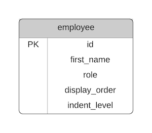
Here’s what the data would look like:

id	first_name	role	display_order	indent_level
1	Claire	CEO	1	0
2	Steve	Head of Sales	2	1
3	Sarah	Head of Support	5	1
4	John	Head of IT	10	1
5	Nathan	Salesperson	3	2
6	Paula	Salesperson	4	2
7	Anne	Customer Support Officer	6	2
8	Roger	Customer Support Officer	7	2
9	Tim	Customer Support Officer	8	2
10	Peter	Assistant	9	2
11	Hugo	Team Leader	11	2
12	Matthew	Developer	12	3
13	Ruth	Developer	13	3
14	Simon	QA Engineer	14	3

Let’s take a look at how we select from and update this data.

 

Selecting the Tree

Selecting from this table is fairly easy. To select all of the data, our query looks like this:

SELECT id, first_name, role, indent_level
FROM employee
ORDER BY display_order;

The results are:

id	first_name	role	indent_level
1	Claire	CEO	0
2	Steve	Head of Sales	1
5	Nathan	Salesperson	2
6	Paula	Salesperson	2
3	Sarah	Head of Support	1
7	Anne	Customer Support Officer	2
8	Roger	Customer Support Officer	2
9	Tim	Customer Support Officer	2
10	Peter	Assistant	2
4	John	Head of IT	1
11	Hugo	Team Leader	2
12	Matthew	Developer	3
13	Ruth	Developer	3
14	Simon	QA Engineer	3

The indent_level can be used for displaying data in a certain way in the application.

 

Select Part of the Tree

If you only want to select a part of the tree, you can filter based on the ID of the record.

For example, to select all employees in the Support department, we can filter on an ID of 3. We’ll also need to exclude those who are displayed after the Head of Support in the tree.

SELECT id, first_name, role, indent_level
FROM employee
WHERE display_order >= (
  SELECT display_order
  FROM employee
WHERE id = 3)
AND display_order < (
  SELECT display_order
  FROM employee
  WHERE indent_level = (
    SELECT indent_level
    FROM employee
    WHERE id = 3
  )
  AND display_order > (
    SELECT display_order
    FROM employee
    WHERE id = 3
  )
)
ORDER BY display_order;

The query is a bit more complex because we are selecting all records that are displayed on or after the Head of Support (id 3), and also only showing records that are displayed before the next record in the tree, which is found by finding the next record at the same indent level.

The results are:

id	first_name	role	indent_level
3	Sarah	Head of Support	1
7	Anne	Customer Support Officer	2
8	Roger	Customer Support Officer	2
9	Tim	Customer Support Officer	2
10	Peter	Assistant	2

 

Adding Records

Adding new records is a little harder. Adding the indent_level is often easy, as we know that before we insert. But adding the display_order is a bit harder as we need to increment all display_order values after the record we want to add.

Let’s say we have a new employee with the following values:

• id: 15
• First Name: Alex
• Role: Salesperson
• Manager: Steve (id 2)

This new record will have a display_order value of 5 and an indent_level of 2.

We need to update the table to make space for this new record:

UPDATE employee
SET display_order = display_order + 1
WHERE display_order >= 5;

We can then insert our new row.

INSERT INTO employee (id, first_name, role, display_order, indent_level)
VALUES (15, 'Alex', 'Salesperson', 5, 2);

Our table now looks like this:

SELECT id, first_name, role, indent_level
FROM employee
ORDER BY display_order;

id	first_name	role	indent_level
1	Claire	CEO	0
2	Steve	Head of Sales	1
5	Nathan	Salesperson	2
6	Paula	Salesperson	2
15	Alex	Salesperson	2
3	Sarah	Head of Support	1
7	Anne	Customer Support Officer	2
8	Roger	Customer Support Officer	2
9	Tim	Customer Support Officer	2
10	Peter	Assistant	2
4	John	Head of IT	1
11	Hugo	Team Leader	2
12	Matthew	Developer	3
13	Ruth	Developer	3
14	Simon	QA Engineer	3

It’s not as easy as the Adjacency List, but easier than Nested Sets.

 

Moving Records

To move records, you’ll also need to update the display_order and indent_level for the records in a specific range, and also the record you’re moving.

For example, if the employee Peter (id 10) moves from Support to Sales, we need to work out the display_order for the record (from 9 to 6) and then update the display order for records in that range.

UPDATE employee
SET display_order = display_order + 1
WHERE display_order <= 9
AND display_order >= 6;

Then we update the display_order for the record we are moving.

UPDATE employee
SET display_order = 6
WHERE id = 10;

It’s not too difficult to move a row in this design.

 

Deleting Records

Deleting records is quite easy. We don’t need to have a continuous range of records, and there’s no relationship to other records to worry about. The indenting and display order will still work.

DELETE FROM employee
WHERE id = 14;

The record is deleted and the other queries we have still work.

 

Pros

Here are the advantages of this Flat Table design:

• Fast for selecting data in a certain way.
• Works well for designs where relationships to parents don’t need to be stored (e.g. forum comments)
• Deleting rows is pretty easy.

 

Cons

Here are the disadvantages of this design:

• Harder to update or add new records, and may be slower to do this with more records.
• Only works for a specific use case

 

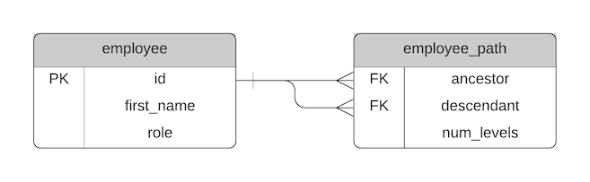
Bridge Table or Closure Table

The Bridge Table design, or Closure Table design, is where a separate table is used that stores the relationships between each record.

It was popularised years ago when it was difficult to work with Adjacency List designs due to the lack of WITH clauses and CONNECT BY keywords in database vendors. It’s simpler to work with than Nested Sets so it’s seen as a good alternative.

How does it work?

It involves creating a new table that stores a row for each record that has an ancestor and descendent relationship. This means we store rows for immediate parents and children as well as those separated by multiple levels in the hierarchy. We also add a row to represent the record’s relationship with itself.

Our new table has the following columns:

• ancestor: the employee id higher in the hierarchy
• descendant: the employee id lower in the hierarchy
• num_levels: the number of levels between the ancestor and descendant (not the root level and descendant)

The ancestor and descendant columns are foreign keys to the employee ID column.

As a reminder, our employee example looks like this:

• Claire
  • Steve
    • Nathan
    • Paula
  • Sarah
    • Anne
    • Roger
    • Tim
    • Peter
  • John
    • Hugo
      • Matthew
      • Ruth
      • Simon

We can apply the Bridging Table or Closure Table concept to our employee table:

Here’s what the data would look like.

id	first_name	role
1	Claire	CEO
2	Steve	Head of Sales
3	Sarah	Head of Support
4	John	Head of IT
5	Nathan	Salesperson
6	Paula	Salesperson
7	Anne	Customer Support Officer
8	Roger	Customer Support Officer
9	Tim	Customer Support Officer
10	Peter	Assistant
11	Hugo	Team Leader
12	Matthew	Developer
13	Ruth	Developer
14	Simon	QA Engineer

Our employee table remains unchanged.

Our new table, which we can call employee_path, looks like this:

ancestor	descendant	num_levels
1	1	0
1	2	1
1	3	1
1	4	1
1	5	2
1	6	2
1	7	2
1	8	2
1	9	2
1	10	2
1	11	2
1	12	3
1	13	3
1	14	3
2	2	0
2	5	1
2	6	1
5	5	0
6	6	0
3	3	0
3	7	1
3	8	1
3	9	1
3	10	1
7	7	0
8	8	0
9	9	0
10	10	0
4	4	0
4	11	1
4	12	2
4	13	2
4	14	2
11	11	0
11	12	1
11	13	1
11	14	1
12	12	0
13	13	0
14	14	0

It has records representing each row’s relationship with any employees under it, as well as a row for itself (where the ancestor equals the descendant).

We’ve now set up our tables. How do we work with them?

 

Selecting the Tree

To select all records in the tree, we join the employee table to the employee_path table where the ancestor is 1 (which is the top level of the tree):

SELECT e.id, e.first_name, e.role
FROM employee e
INNER JOIN employee_path p ON e.id = p.descendant
WHERE p.ancestor = 1;

The results are:

id	first_name	role
1	Claire	CEO
2	Steve	Head of Sales
3	Sarah	Head of Support
4	John	Head of IT
5	Nathan	Salesperson
6	Paula	Salesperson
7	Anne	Customer Support Officer
8	Roger	Customer Support Officer
9	Tim	Customer Support Officer
10	Peter	Assistant
11	Hugo	Team Leader
12	Matthew	Developer
13	Ruth	Developer
14	Simon	QA Engineer

We can see all of the employees here. We could also include the num_levels column in the output, if we wanted to see the level of that item in the tree.

This demonstrates the reason we have a row for the employee ID in both the ancestor and descendant rows. If it was not there, it would not appear in this result.

 

Select Part of the Tree

To select only part of the tree, we can run the same query with a different value in the WHERE clause.

For example, to select all employees in the Support department, we can filter on an ID of 3.

SELECT e.id, e.first_name, e.role
FROM employee e
INNER JOIN employee_path p ON e.id = p.descendant
WHERE p.ancestor = 3;

The results are:

id	first_name	role
3	Sarah	Head of Support
7	Anne	Customer Support Officer
8	Roger	Customer Support Officer
9	Tim	Customer Support Officer
10	Peter	Assistant

The SELECT query is pretty simple to get the data you need.

 

Adding Records

Inserting a new row in this design takes a couple of steps.

First, you need to insert a row that references itself (a row where the ancestor and descendent is the same).

Then, you need to insert rows that reference the new row’s parent but refer to your new row as well.

Let’s say we have a new employee with the following values:

• id: 15
• First Name: Alex
• Role: Salesperson
• Manager: Steve (id 2)

We’ll need to insert a new row in the employee table:

INSERT INTO employee (id, first_name, role)
VALUES (15, 'Alex', 'Salesperson');

We’ll also need to insert a new record into the employee_path table for this record:

INSERT INTO employee_path (ancestor, descendant, num_levels)
VALUES (15, 15, 0);

Next, we need to insert records to represent the new employee’s parent record and all of its ancestors. This means ID 2 (Steve) and ID 1 (Claire).

We can do this easily by querying the table for all records where the descendant is the new employee’s manager:

SELECT ancestor, descendant, num_levels
FROM employee_path
WHERE descendant = 2;

This will show these results:

ancestor	descendant	num_levels
1	2	1
2	2	0

We need to insert new rows with these ancestor values, a descendant value of our new ID (15), and a num_levels of the existing value + 1 (as the new record is a child of ID 2).

The query to do this is:

INSERT INTO employee_path (ancestor, descendant, num_levels)
SELECT ancestor, 15, num_levels + 1
FROM employee_path
WHERE descendant = 2;

Our new records will be added to this table, which will show up when we select the full tree again.

 

Moving Records

Moving records is a bit tricky in this design.

To move a record, we need to:

• Delete rows from the employee_path that refer to the ID in the tree
• Insert new rows to place the employee in the new position in the tree

For example, if the employee Peter (id 10) moves from Support (id 3) to Sales (id 2), we take the following steps.

First, we delete records that share the same descendants (records higher up in the tree).

DELETE FROM employee_path
WHERE descendant IN (
  SELECT descendant
  FROM employee_path
  WHERE ancestor = 3
)
AND ancestor IN (
  SELECT ancestor
  FROM employee_path
  WHERE descendant = 3
  AND ancestor != descendant
);

We’ve added the ancestor != descendant because we don’t want to remove the self-referencing record from the table.

Next, we add the record that’s moving to the new location:

INSERT INTO employee_path
SELECT a.ancestor, b.descendant
FROM employee_path a
CROSS JOIN employee_path b
WHERE a.descendant = 2
AND b.ancestor = 10;

We’ve used a cross join to get all possible combinations of values, which are then used to create the new tree values.

 

Deleting Records

To delete a record, we delete the record from the employee table. We also need to delete all records from the employee_path table that have the deleted ID as a descendant.

For example, to delete employee 14:

DELETE FROM employee
WHERE id = 14;
DELETE FROM employee_path
WHERE descendant = 14;

If the record has any descendants, you’ll need to delete all records in employee_path that have those descendants too.

DELETE FROM employee_path
WHERE descendant IN (
  SELECT descendant
  FROM employee_path
  WHERE ancestor = 14
);

 

Pros

Here are some advantages of the Bridge Table or Closure Table design:

• Cleaner than the Nested Sets design.
• Easy to select all records or select a subtree
• Fairly easy to add a new record
• Easy to add additional information to the table, such as the number of levels

 

Cons

Here are some disadvantages of the Bridge Table or Closure Table design:

• Hard to move records to another place in the tree
• Hard to delete records from the tree

 

Lineage Column or Path Enumeration

Another design for working with hierarchical data is called Lineage Column, also known as Path Enumeration. This design involves adding a single VARCHAR column to your table that stores a full path from the current record to the root, in a similar way that a directory path works in a file system.

On your computer, you may have a Documents folder. But this folder doesn’t exist on its own on the hard drive. It exists at a point in a directory tree. And the full path name of this folder could be something like “C:\\\\Ben\\\\My Documents\\\\Documents\\\\”.

Using our employee example, the hierarchy looks like this:

• Claire
  • Steve
    • Nathan
    • Paula
  • Sarah
    • Anne
    • Roger
    • Tim
    • Peter
  • John
    • Hugo
      • Matthew
      • Ruth
      • Simon

In our employee table, we add a single column that represents the full path of the record. We’ll call it record_path, just to avoid any issues if the word “path” is a reserved word.

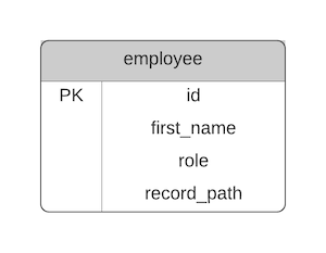
This column stores a string that contains the values of all of its ancestors. The values are the IDs and can be separated a / character or a – character (as long as it’s consistent).

id	first_name	role	record_path
1	Claire	CEO	1/
2	Steve	Head of Sales	1/2/
3	Sarah	Head of Support	1/3/
4	John	Head of IT	1/4/
5	Nathan	Salesperson	1/2/5/
6	Paula	Salesperson	1/2/6/
7	Anne	Customer Support Officer	1/3/7/
8	Roger	Customer Support Officer	1/3/8/
9	Tim	Customer Support Officer	1/3/9/
10	Peter	Assistant	1/3/10/
11	Hugo	Team Leader	1/4/11/
12	Matthew	Developer	1/4/11/12/
13	Ruth	Developer	1/4/11/13/
14	Simon	QA Engineer	1/4/11/14/

 

Selecting the Tree

To select the entire tree, we simply select all data from the table.

SELECT id, first_name, role, record_path
FROM employee;

We can calculate the level of the record by counting the number of “/” characters in the record_path value, or we can add a column that stores this.

You would then use the application to display the records in the right order by transforming the record_path into whatever format is needed.

 

Select Part of the Tree

To select part of the tree, you can query the table to find records where the record_path has a partial match to the area of the tree you want.

For example, to select all employees in the Support department (employee id 3), we can find values that contain the string “1/3/”.

SELECT id, first_name, role, record_path
FROM employee
WHERE record_path LIKE '1/3/%';

This will show these results:

id	first_name	role	record_path
3	Sarah	Head of Support	1/3/
7	Anne	Customer Support Officer	1/3/7/
8	Roger	Customer Support Officer	1/3/8/
9	Tim	Customer Support Officer	1/3/9/
10	Peter	Assistant	1/3/10/

 

Adding Records

Adding new records using this design is pretty simple, and similar to the Adjacency List method.

To add a new record, insert a new record into the employee table. You can copy the record_path from the parent record and add the new ID to the end.

Let’s say we have a new employee with the following values:

• id: 15
• First Name: Alex
• Role: Salesperson
• Manager: Steve (id 2)

We’ll need to insert a new row in the employee table:

INSERT INTO employee (id, first_name, role, record_path)
VALUES (15, 'Alex', 'Salesperson', '1/2/15/');

The record is now in the table and will be included in the queries you write on the table.

 

Moving Records

Moving a record is also quite easy but prone to errors. You’ll need to update the record_path of the record you want to move to replace the path with the new path.

This could be easy if you can manually enter the path, or it could be harder if you need to find a string and replace it. This is because there’s no validation like a foreign key to the related employee records.

For example, if the employee Peter (id 10) moves from Support (id 3) to Sales (id 2), we can update that employee record with the new path. The new path would be “1/2/10/” instead of “1/3/10/”.

UPDATE employee
SET record_path = '1/2/10/'
WHERE id = 10;

The employee will now be in the right place in the hierarchy.

 

Deleting Records

To delete a record with no children, you can simply remove the record from the employee table.

DELETE FROM employee
WHERE id = 14;

If the record you’re deleting has children, you’ll need to update the record_path value for each of the children to remove the id that you’re deleting.

For example, to delete record 11 (which has child records), we need to:

DELETE FROM employee
WHERE id = 11;

UPDATE employee
SET record_path = SUBSTITUTE(record_path, '/11/', '/')
WHERE record_path LIKE '1/4/11/%';

The SUBSTITUTE function here will replace the value of /11/ with just a / character, essentially removing it from the value. You may need to use a different function if SUBSTITUTE is not in your database.

It’s a bit messy and error-prone, but like many of these methods, you can put this functionality inside a stored procedure and then call the stored procedure to make it easier.

 

Pros

Here are the advantages of the Lineage Column or Path Enumeration method:

• Easy to insert new records.
• Easy to select the whole or part of the tree
• Moving records can be easy

 

Cons

Here are the disadvantages of the Lineage Column or Path Enumeration method:

• Deleting records can be hard
• Moving records can be hard in some situations
• There is no referential integrity, which can compromise the quality of your data. This is probably the biggest disadvantage.
• There’s a maximum length of values in the path column, meaning you have a maximum depth of your hierarchy.

 

Summary of Methods

We’ve seen several different methods for implementing hierarchical data. How do they all compare to each other?

This table summarises the differences between each method.

Method	Select	Insert	Update	Delete	Ref. Integ.
Adjacency List	Hard	Easy	Easy	Easy	Yes
Nested Set	Easy	Hard	Hard	Hard	No
Flat Table	Easy	Hard	Easy	Easy	N/A
Bridge Table/Closure Table	Easy	Easy	Hard	Hard	Yes
Lineage Column/Path Enumeration	Easy	Easy	Easy	Hard	No

How do you know which method to implement?

 

Which Method Should I Use?

So there are several ways to store hierarchical data in an SQL database. Which method should you use?

I recommend using the Adjacency List option in most cases.

You could consider the Nested Set if you are mostly selecting from the table and rarely updating or if the SELECT performance of Adjacency List is poor.

The other methods could work in specific cases, but in most cases the Adjacency List will be OK.

 

Conclusion

Hierarchical data isn’t something that is done very often or comes standard with relational databases. Fortunately, there are several ways to implement it, each with its pros and cons.

Consider using the Adjacency List method which will work in most cases, and queries for this are supported in recent versions of each vendor’s database.

If you want an easy-to-use PDF guide for the main features in different database vendors, get my SQL Cheat Sheets here: