Complex SQL Query Example – Daily Order Analysis

If you want to see how to write a complex query on an SQL database, this example will show you.

Introduction

This article is a case study on writing a complex query on an SQL database.

We start with a set of database tables, populated with data.

We then have a requirement to show some data by writing a query.

We’ll write the query step-by-step and get to our final result.

You’ll see how a complex query can be written in smaller pieces, checking the results along the way and making any adjustments.

Let’s get started!

 

Setup

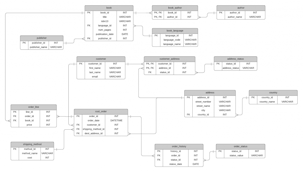
For this case study, we’re using a sample bookstore database. It has books, authors, customers, orders, and several other tables.

Here’s the ERD:

How can you set up this database?

I’ve written an entire post on how to download the SQL files and run them to create and populate this database on your own computer: How to Set Up the Sample Bookstore Database.

The files are available in Oracle, SQL Server, MySQL, and PostgreSQL.

So, feel free to follow along by downloading the scripts in that post.

 

Requirements

What query are we going to write? What are our requirements?

Let’s say we’re in a team and we have a Product Owner who wants a report to be created.

The Product Owner wants this report to show a daily order tally. They want to see:

• the order date
• the number of orders for that date
• the number of books ordered
• the total price of the orders
• the running total of books for the month
• the number of books from the same day last week (e.g. how this Sunday compares to last Sunday)

These totals should also show for each month and overall.

This sounds complicated! If you’re looking at this list you might be thinking some of it looks simple and may have some ideas on how to do it.

Other parts may not be simple.

Let’s get started with writing a query.

In this example, we’ll use MySQL. I’ll aim to use standard syntax where possible, but explain any differences that may apply to other databases.

 

Start Our Query

We first need to load the sample database. I’ll assume you’ve done that. If not, you can follow the steps in this post: How to Set Up the Sample Bookstore Database.

Our requirement was to show the order date and a range of totals. Let’s start by showing the order date.

It doesn’t seem like much, but it’s good to start with a simple query and build on it from there.

SELECT order_date
FROM cust_order;

Here are the results. I’m showing part of the results rather than the full results as there are too many.

order_date

2019-11-01 20:09:41

2019-02-28 21:52:56

2018-11-07 3:42:37

2018-12-29 2:57:14

2021-07-02 8:07:49

2019-11-30 17:17:25

2021-02-24 0:44:31

2019-12-08 11:52:51

2018-09-20 12:27:23

2018-07-18 19:08:46

2020-03-04 21:03:57

We can see the order_date from this table. The column shows both the date and time, which is good to know.

The data is in what looks like a random order. Let’s order the results by the order_date.

SELECT order_date
FROM cust_order
ORDER BY order_date ASC;

Here are the results.

order_date

2018-07-10 15:59:58

2018-07-10 16:42:01

2018-07-10 21:54:06

2018-07-10 23:14:06

2018-07-11 1:52:01

2018-07-11 3:33:18

2018-07-11 8:14:25

2018-07-11 11:46:18

2018-07-11 12:01:24

2018-07-12 0:12:36

2018-07-12 2:48:02

The cust_order records are ordered by the order_date.

 

Show Number of Orders Per Date

We can see the order dates. Now we need to show the number of orders per date.

Whenever we need to see something like “the number of X per Y”, it usually means we need to use an aggregate function and group the results.

In this example, we want to see the number of orders, so we use the COUNT function.

Our query can be changed to this:

SELECT
order_date,
COUNT(*)
FROM cust_order
ORDER BY order_date ASC;

If we run this query in MySQL, this is what we’ll get:

order_date	COUNT(*)
2021-01-14 21:43:50	7550

If we run this in other databases, we’ll get an error about a missing GROUP BY clause.

The issue with the MySQL result is that it shows a single row and a count for all records. There are no errors shown, and the count is not actually the count of records for that date.

It’s a dangerous result, but we can easily fix it by adding a GROUP BY.

SELECT
order_date,
COUNT(*)
FROM cust_order
GROUP BY order_date
ORDER BY order_date ASC;

Here are the results.

order_date	COUNT(*)
2018-07-10 15:59:58	1
2018-07-10 16:42:01	1
2018-07-10 21:54:06	1
2018-07-10 23:14:06	1
2018-07-11 1:52:01	1
2018-07-11 3:33:18	1
2018-07-11 8:14:25	1
2018-07-11 11:46:18	1
2018-07-11 12:01:24	1
2018-07-12 0:12:36	1
2018-07-12 2:48:02	1

In this result, we can see dates and counts. However, it’s showing multiple rows for orders on the same day. We can see 4 orders on 2018-07-10.

(Your results may be different because the order dates are randomised. But you should still see a similar output).

Why isn’t it grouping properly?

It is grouping, but it’s grouping on the order_date field, which includes the date and the time, down to the second. If there are two orders that are created at the same second, the count will be 2, otherwise it will be 1.

We need to change the query to show only the date and not the time.

We can do this in several ways. One way is the DATE_FORMAT function.

We can use the DATE_FORMAT function to only show the date, and then group by that new field.

SELECT
DATE_FORMAT(order_date, '%Y-%m-%d'),
COUNT(*)
FROM cust_order
GROUP BY DATE_FORMAT(order_date, '%Y-%m-%d')
ORDER BY order_date ASC;

We’re grouping by the same field that we’re selecting. Here are the results.

DATE_FORMAT( order_date, ‘%Y-%m-%d’)	COUNT(*)
2018-07-10	4
2018-07-11	5
2018-07-12	5
2018-07-13	7
2018-07-14	7
2018-07-15	4
2018-07-16	5
2018-07-17	5

Better! We can see the number of orders for each date, and each date is only showing once.

What about those column headings? They are messy, the first one is long, and they don’t really describe what we’re seeing.

Fortunately, we can use a feature called a column alias to rename them.

Let’s do that now. We can add the word AS after the column, then add a new name.

SELECT
DATE_FORMAT(order_date, '%Y-%m-%d') AS order_day,
COUNT(*) AS num_orders
FROM cust_order
GROUP BY DATE_FORMAT(order_date, '%Y-%m-%d')
ORDER BY order_date ASC;

Here are the results.

order_day	num_orders
2018-07-10	4
2018-07-11	5
2018-07-12	5
2018-07-13	7
2018-07-14	7
2018-07-15	4
2018-07-16	5
2018-07-17	5

The data is the same and the headings are much clearer and easier to read. We have the order_day, which is the date, and num_orders which is the number of orders for that day.

Let’s look at the next part of the query.

 

Add Number of Books Ordered

The next requirement to add is to “show the number of books ordered”.

How do we do this?

We can take a look at our cust_order table to see what’s in it:

SELECT *
FROM cust_order;

The results are:

order_id	order_date	customer_id	shipping_method_id	dest_address_id
1	2021-01-14 21:43:50	343	2	1
2	2020-11-20 17:10:32	892	1	2
3	2019-11-01 20:09:41	1078	3	2
4	2019-02-28 21:52:56	1652	4	2
5	2018-11-07 3:42:37	1823	4	2
6	2018-12-29 2:57:14	32	3	4
7	2021-07-02 8:07:49	347	3	4
8	2019-11-30 17:17:25	1409	1	4
9	2021-02-24 0:44:31	1569	1	4
10	2019-12-08 11:52:51	1628	1	4

There are a few fields here, but nothing that indicates the number of books ordered.

Let’s take a look at our ERD to see how cust_order is related to books:

We can see that the order_line table is related to cust_order. It seems there are many order_line rows for one cust_order row. The order_line table also has a book_id column which links to the book table.

So, it seems there is one order_line for each book in an order.

We can check what’s in the table by selecting all columns for a single order_line. I’ll pick order ID 3 just as an example.

SELECT *
FROM order_line
WHERE order_id = 3;

The results are:

line_id	order_id	book_id	price
4073	3	465	6.72
12115	3	1486	2.51

We can see that order ID 3 has two records, which means it includes two books.

We can include this information from this table in our main query to get the number of books.

Here’s our updated query:

SELECT
DATE_FORMAT(co.order_date, '%Y-%m-%d') AS order_day,
COUNT(co.order_id) AS num_orders
FROM cust_order co
INNER JOIN order_line ol ON co.order_id = ol.order_id
GROUP BY DATE_FORMAT(co.order_date, '%Y-%m-%d')
ORDER BY co.order_date ASC;

We’ve done a couple of things:

• We used an INNER JOIN to join the cust_order table to the order_line table.
• We’ve added a table alias to both tables: “co” for cust_order and “ol” for order_line.

We haven’t added any columns to show the number of books yet.

Let’s run the query and see what it shows.

order_day	num_orders
2018-07-10	12
2018-07-11	8
2018-07-12	8
2018-07-13	12
2018-07-14	17
2018-07-15	8
2018-07-16	10
2018-07-17	8

Hmm. There seems to be an issue with the num_orders here. If we refer back to the previous query results, we could see the numbers were lower:

order_day	num_orders
2018-07-10	4
2018-07-11	5
2018-07-12	5
2018-07-13	7
2018-07-14	7
2018-07-15	4
2018-07-16	5
2018-07-17	5

They have increased for all dates, and by different amounts.

Why did this happen?

The first thing I do when looking for issues in data is to look at a specific row. So, let’s choose a specific date and see the orders for the date.

SELECT
co.*,
ol.*
FROM cust_order co
INNER JOIN order_line ol ON co.order_id = ol.order_id
WHERE DATE_FORMAT(co.order_date, '%Y-%m-%d') = '2018-07-10';

We select data from both tables for the first date: 2018-07-10.

order_id	order_date	customer_id	shipping_method_id	dest_address_id	line_id	order_id	book_id	price
1147	2018-07-10 15:59:58	237	3	416	875	1147	3722	16.18
1147	2018-07-10 15:59:58	237	3	416	8512	1147	5328	5.27
1147	2018-07-10 15:59:58	237	3	416	14800	1147	7652	5.16
1287	2018-07-10 21:54:06	475	3	472	1818	1287	4661	19.05
1287	2018-07-10 21:54:06	475	3	472	12396	1287	5241	6.22
1287	2018-07-10 21:54:06	475	3	472	15627	1287	8621	15.27
9218	2018-07-10 23:14:06	32	3	4	130	9218	10473	17.74
9218	2018-07-10 23:14:06	32	3	4	10682	9218	8532	16.82
9218	2018-07-10 23:14:06	32	3	4	15403	9218	7296	5.22
9234	2018-07-10 16:42:01	1023	4	10	3876	9234	233	18.51
9234	2018-07-10 16:42:01	1023	4	10	9769	9234	4259	5.94
9234	2018-07-10 16:42:01	1023	4	10	15331	9234	11050	11.2

Looking at this data, we can see 12 rows. The original query showed 4 orders and the updated query showed 12 orders.

The data shows that there are 4 different order_id values and 12 different book_id values.

Aah, that’s why.

Our COUNT function is counting all rows in the result set. It used to have 4 rows, but when we joined to the order_line table, more rows were added, bringing the COUNT up to 12.

For the count of orders, we only want to see the unique order IDs. We can do this using the DISTINCT keyword inside the COUNT function.

SELECT
DATE_FORMAT(co.order_date, '%Y-%m-%d') AS order_day,
COUNT(DISTINCT co.order_id) AS num_orders
FROM cust_order co
INNER JOIN order_line ol ON co.order_id = ol.order_id
GROUP BY DATE_FORMAT(co.order_date, '%Y-%m-%d')
ORDER BY co.order_date ASC;

Here are our results:

order_day	num_orders
2018-07-10	4
2018-07-11	5
2018-07-12	5
2018-07-13	7
2018-07-14	7
2018-07-15	4
2018-07-16	5
2018-07-17	5

Much better. The numbers for each day look like the values we had earlier.

Now we need to add in the number of books ordered on each day. We can do this by adding a COUNT function and count the number of records in the order_line table.

We could actually count any column, as they should all be the same, but it’s usually better to count the primary key as it’s not going to be NULL (and NULL values can impact aggregate functions).

Here’s our updated query:

SELECT
DATE_FORMAT(co.order_date, '%Y-%m-%d') AS order_day,
COUNT(DISTINCT co.order_id) AS num_orders,
COUNT(ol.book_id) AS num_books
FROM cust_order co
INNER JOIN order_line ol ON co.order_id = ol.order_id
GROUP BY DATE_FORMAT(co.order_date, '%Y-%m-%d')
ORDER BY co.order_date ASC;

We’ve added a COUNT function on the ol.book_id column, and given it an alias of num_books.

Here are the results.

order_day	num_orders	num_books
2018-07-10	4	12
2018-07-11	5	8
2018-07-12	5	8
2018-07-13	7	12
2018-07-14	7	17
2018-07-15	4	8
2018-07-16	5	10
2018-07-17	5	8

The num_orders is the same as earlier, and the num_books has been added. This shows that, for example on 2018-07-10, there were 4 orders for a total of 12 books.

 

Add Total Price of the Books

The next requirement to add to our query is to show the total price of books sold.

Where is this field located? If we have a look at the ERD, we can see a price column in the order_line table. This represents the price that the book was sold for in the order.

So, we can add this to our query. To get the total price, we can use the SUM function on this price column.

SELECT
DATE_FORMAT(co.order_date, '%Y-%m-%d') AS order_day,
COUNT(DISTINCT co.order_id) AS num_orders,
COUNT(ol.book_id) AS num_books,
SUM(ol.price) AS total_price
FROM cust_order co
INNER JOIN order_line ol ON co.order_id = ol.order_id
GROUP BY DATE_FORMAT(co.order_date, '%Y-%m-%d')
ORDER BY co.order_date ASC;

Here are the results.

order_day	num_orders	num_books	total_price
2018-07-10	4	12	142.58
2018-07-11	5	8	60.43
2018-07-12	5	8	97.84
2018-07-13	7	12	99.27
2018-07-14	7	17	163.27
2018-07-15	4	8	78.24
2018-07-16	5	10	131.93
2018-07-17	5	8	80.63

Our query is looking good so far! Let’s see what’s next.

 

Add a Running Total

The next requirement was to see “the running total of books for the month”.

A running total means a sum of orders for the current row and all rows before it. This means each row the running total should increase.

The “for the month” part of the requirement indicates that it should reset at the start of the next month.

How do we do that in SQL?

First, it would be helpful to see the month of each order. We can see the date which includes the month, but showing the month may make it easier to visualise.

SELECT
DATE_FORMAT(co.order_date, '%Y-%m') AS order_month,
DATE_FORMAT(co.order_date, '%Y-%m-%d') AS order_day,
COUNT(DISTINCT co.order_id) AS num_orders,
COUNT(ol.book_id) AS num_books,
SUM(ol.price) AS total_price
FROM cust_order co
INNER JOIN order_line ol ON co.order_id = ol.order_id
GROUP BY 
  DATE_FORMAT(co.order_date, '%Y-%m'),
  DATE_FORMAT(co.order_date, '%Y-%m-%d')
ORDER BY co.order_date ASC;

We’ve added a new column with an alias of order_month to the SELECT clause. This uses the date_format function to just get the month and year. We also add this to the GROUP BY clause so the query results are shown correctly.

Here are the results.

order_month	order_day	num_orders	num_books	total_price
2018-07	2018-07-10	4	12	142.58
2018-07	2018-07-11	5	8	60.43
2018-07	2018-07-12	5	8	97.84
2018-07	2018-07-13	7	12	99.27
2018-07	2018-07-14	7	17	163.27
2018-07	2018-07-15	4	8	78.24
2018-07	2018-07-16	5	10	131.93
2018-07	2018-07-17	5	8	80.63

We’ve got the month. Now we need to add the running total.

In SQL, many functions perform calculations on data in the same row, such as rounding a number, or over all data in a table, such as counting rows.

Another way to look at data for a function is a subset of your results. This is often referred to as a “window”, and it’s what we want to do here. We want to get a total for each row, but the total should only include records that:

• Appear before the current record in the results (records with an earlier order_day)
• Are in the same month (have the same order_month)

We can do this using analytic functions or window functions. I’ve written a guide here if you want to know more.

How do we know we need analytic functions? Because of the data we want to include in the total. We need more than just one row, but not all rows in the result.

So, let’s do this now. We need to add a COUNT function because we are counting the number of books.

SELECT
DATE_FORMAT(co.order_date, '%Y-%m') AS order_month,
DATE_FORMAT(co.order_date, '%Y-%m-%d') AS order_day,
COUNT(DISTINCT co.order_id) AS num_orders,
COUNT(ol.book_id) AS num_books,
SUM(ol.price) AS total_price,
COUNT(ol.book_id) OVER (ORDER BY DATE_FORMAT(co.order_date, '%Y-%m-%d')) AS running_total_num_books
FROM cust_order co
INNER JOIN order_line ol ON co.order_id = ol.order_id
GROUP BY
DATE_FORMAT(co.order_date, '%Y-%m'),
DATE_FORMAT(co.order_date, '%Y-%m-%d')
ORDER BY co.order_date ASC;

We’ve added in one column into our SELECT clause:

COUNT(ol.book_id) OVER (ORDER BY DATE_FORMAT(co.order_date, '%Y-%m-%d')) AS running_total_num_books

Let’s break this down as it looks complicated.

We’ve started with a COUNT function, and we’re counting the number of books, so we’ve used the ol.book_id column.

Next, we’ve added the OVER keyword. This allows us to use COUNT as an analytic function. OVER will let us specify how we want to create subsets or windows of data.

Inside the brackets after OVER, we add an ORDER BY clause. This only specifies the order of data used for the COUNT function, not the overall result. The ordering is needed here so the COUNT function knows which records come before it.

We’ve ordered by the DATE_FORMAT function of the order_date column, which is saying “order by order date”.

We then give it a column alias of running_total_num_books.

Let’s see the results.

order_month	order_day	num_orders	num_books	total_price	running_total_num_books
2018-07	2018-07-10	4	12	142.58	1
2018-07	2018-07-11	5	8	60.43	2
2018-07	2018-07-12	5	8	97.84	3
2018-07	2018-07-13	7	12	99.27	4
2018-07	2018-07-14	7	17	163.27	5
2018-07	2018-07-15	4	8	78.24	6
2018-07	2018-07-16	5	10	131.93	7
2018-07	2018-07-17	5	8	80.63	8

Hmm… it seems we have a problem. We see in the running_total_num_books column that the number starts at 1 and increases by 1 for each row. We were expecting the running number of books, which would be 12 then 20 then 28.

What’s the issue here?

Our function says COUNT(ol.book_id). This means we are counting the book_id values for each row in our result. It’s the same as counting the number of rows here.

What we want to do is look at that num_books column and SUM those values.

We want to see the SUM of the num_books value for all rows before the current row in the month.

So, we can change our query to put a SUM function around the COUNT function in the new column we added.

Why do we add a SUM around the COUNT? Because the num_books is calculated as COUNT(ol.book_id) and we want to SUM that value.

We can look at our results after the query and see if it is correct.

Here’s the updated query.

SELECT
DATE_FORMAT(co.order_date, '%Y-%m') AS order_month,
DATE_FORMAT(co.order_date, '%Y-%m-%d') AS order_day,
COUNT(DISTINCT co.order_id) AS num_orders,
COUNT(ol.book_id) AS num_books,
SUM(ol.price) AS total_price,
SUM(COUNT(ol.book_id)) OVER (
  ORDER BY DATE_FORMAT(co.order_date, '%Y-%m-%d')
) AS running_total_num_books
FROM cust_order co
INNER JOIN order_line ol ON co.order_id = ol.order_id
GROUP BY 
  DATE_FORMAT(co.order_date, '%Y-%m'),
  DATE_FORMAT(co.order_date, '%Y-%m-%d')
ORDER BY co.order_date ASC;

And here are the results.

order_month	order_day	num_orders	num_books	total_price	running_total_num_books
2018-07	2018-07-10	4	12	142.58	12
2018-07	2018-07-11	5	8	60.43	20
2018-07	2018-07-12	5	8	97.84	28
2018-07	2018-07-13	7	12	99.27	40
2018-07	2018-07-14	7	17	163.27	57
2018-07	2018-07-15	4	8	78.24	65
2018-07	2018-07-16	5	10	131.93	75
2018-07	2018-07-17	5	8	80.63	83

What happens when we get to orders at the end of the month? Here are the same results for a different date range:

order_month	order_day	num_orders	num_books	total_price	running_total_num_books
2018-07	2018-07-27	8	19	158.55	252
2018-07	2018-07-28	4	5	39.67	257
2018-07	2018-07-29	6	13	112.74	270
2018-07	2018-07-30	3	9	101.07	279
2018-07	2018-07-31	6	11	103.81	290
2018-08	2018-08-01	11	19	223.68	309
2018-08	2018-08-02	8	18	174.99	327
2018-08	2018-08-03	5	11	145.77	338
2018-08	2018-08-04	4	8	79.42	346

We can see that on 2018-08-01, the running_total_num_books value continues to increase. It did not reset back to 0 or the total of the num_books for that day.

This is because we didn’t specify in our COUNT function that it should only consider rows in the current month.

How can we update our query?

We add a PARTITION BY clause to our function. This is another feature of analytic functions.

We use the PARTITION BY clause to specify the window or partition that the function should be calculated over.

We want to partition by the month of the order date, so we update our query to look like this:

SELECT
DATE_FORMAT(co.order_date, '%Y-%m') AS order_month,
DATE_FORMAT(co.order_date, '%Y-%m-%d') AS order_day,
COUNT(DISTINCT co.order_id) AS num_orders,
COUNT(ol.book_id) AS num_books,
SUM(ol.price) AS total_price,
SUM(COUNT(ol.book_id)) OVER (
  PARTITION BY DATE_FORMAT(co.order_date, '%Y-%m')
  ORDER BY DATE_FORMAT(co.order_date, '%Y-%m-%d')
) AS running_total_num_books
FROM cust_order co
INNER JOIN order_line ol ON co.order_id = ol.order_id
GROUP BY 
  DATE_FORMAT(co.order_date, '%Y-%m'),
  DATE_FORMAT(co.order_date, '%Y-%m-%d')
ORDER BY co.order_date ASC;

You can see the new PARTITION BY clause in the query here. Let’s see the results again:

order_month	order_day	num_orders	num_books	total_price	running_total_num_books
2018-07	2018-07-10	4	12	142.58	12
2018-07	2018-07-11	5	8	60.43	20
2018-07	2018-07-12	5	8	97.84	28
2018-07	2018-07-13	7	12	99.27	40
2018-07	2018-07-14	7	17	163.27	57
2018-07	2018-07-15	4	8	78.24	65
2018-07	2018-07-16	5	10	131.93	75
2018-07	2018-07-17	5	8	80.63	83

And here are the results for the start of the next month.

order_month	order_day	num_orders	num_books	total_price	running_total_num_books
2018-07	2018-07-27	8	19	158.55	252
2018-07	2018-07-28	4	5	39.67	257
2018-07	2018-07-29	6	13	112.74	270
2018-07	2018-07-30	3	9	101.07	279
2018-07	2018-07-31	6	11	103.81	290
2018-08	2018-08-01	11	19	223.68	19
2018-08	2018-08-02	8	18	174.99	37
2018-08	2018-08-03	5	11	145.77	48
2018-08	2018-08-04	4	8	79.42	56

Aha! We can see that the running total has been reset at the start of the next month! We can also see in the first results table that the running total has begun correctly.

 

Reformat Query

Let’s take a look at our query again.

SELECT
DATE_FORMAT(co.order_date, '%Y-%m') AS order_month,
DATE_FORMAT(co.order_date, '%Y-%m-%d') AS order_day,
COUNT(DISTINCT co.order_id) AS num_orders,
COUNT(ol.book_id) AS num_books,
SUM(ol.price) AS total_price,
SUM(COUNT(ol.book_id)) OVER (
  PARTITION BY DATE_FORMAT(co.order_date, '%Y-%m')
  ORDER BY DATE_FORMAT(co.order_date, '%Y-%m-%d')
) AS running_total_num_books
FROM cust_order co
INNER JOIN order_line ol ON co.order_id = ol.order_id
GROUP BY 
  DATE_FORMAT(co.order_date, '%Y-%m'),
  DATE_FORMAT(co.order_date, '%Y-%m-%d')
ORDER BY co.order_date ASC;

You may be thinking that it’s getting a bit repetitive. We’ve used the DATE_FORMAT function to format the date 6 times, formatting as both the day and the month 3 times.

Is there a way we can clean this up?

Fortunately, there is. It’s a technique I often use to make queries simpler to write and edit.

We’re going to move the calculation of the columns into a subquery, and then select those columns to show what we need.

First, we write the subquery, which formats the dates how we want.

SELECT
DATE_FORMAT(co.order_date, '%Y-%m') AS order_month,
DATE_FORMAT(co.order_date, '%Y-%m-%d') AS order_day,
co.order_id,
ol.book_id,
ol.price
FROM cust_order co
INNER JOIN order_line ol ON co.order_id = ol.order_id;

It also includes the IDs and price that we need.

Next, we select the fields that we want from this query as a subquery. This includes the fields to show, the aggregate functions, and the analytic functions.

SELECT
order_month,
order_day,
COUNT(DISTINCT order_id) AS num_orders,
COUNT(book_id) AS num_books,
SUM(price) AS total_price,
SUM(COUNT(book_id)) OVER (
PARTITION BY order_month
ORDER BY order_day
) AS running_total_num_books
FROM (
  SELECT
  DATE_FORMAT(co.order_date, '%Y-%m') AS order_month,
  DATE_FORMAT(co.order_date, '%Y-%m-%d') AS order_day,
  co.order_id,
  ol.book_id,
  ol.price
  FROM cust_order co
  INNER JOIN order_line ol ON co.order_id = ol.order_id
) sub
GROUP BY order_month, order_day
ORDER BY order_day ASC;

The query is a little longer, but we’re only formatting the dates in one place, and selecting and ordering them is much easier.

We still see the same data when we run this query.

 

Add Number from Last Week

What’s the next requirement?

It’s to show “the number of books from the same day last week (e.g. how this Sunday compares to last Sunday)”

So we need to:

• look at a row
• determine the row that represents the sales from 7 days ago
• get the number of books from that row

It sounds complicated. How can we do this?

We can use functions that are standard in SQL called LEAD and LAG.

LEAD lets you get data from rows further down in the results, and LAG lets you get data from rows further up in the results.

As we’re ordering by order date in ascending order, the earlier orders are further up the results, so we can use LAG.

We use LAG to get a value from an order date from one week ago, or seven days.

LAG is used as an analytic function, so we specify the OVER clause and the ORDER BY clause to define how the data is searched.

SELECT
order_month,
order_day,
COUNT(DISTINCT order_id) AS num_orders,
COUNT(book_id) AS num_books,
SUM(price) AS total_price,
SUM(COUNT(book_id)) OVER (
  PARTITION BY order_month
  ORDER BY order_day
) AS running_total_num_books,
LAG(COUNT(book_id), 1) OVER (ORDER BY order_day) AS prev_books
FROM (
  SELECT
  DATE_FORMAT(co.order_date, '%Y-%m') AS order_month,
  DATE_FORMAT(co.order_date, '%Y-%m-%d') AS order_day,
  co.order_id,
  ol.book_id,
  ol.price
  FROM cust_order co
  INNER JOIN order_line ol ON co.order_id = ol.order_id
) sub
GROUP BY order_month, order_day
ORDER BY order_day ASC;

In this query, we’ve added the LAG function.

LAG(COUNT(book_id), 1) OVER (ORDER BY order_day) AS prev_books

Inside the LAG function, we are looking for the count of the book ID. The next parameter of 1 is the number of rows to go back up the result set. We’re using 1 just to test that it works, and we can adjust later.

We then add the OVER clause, and an ORDER BY, which specifies that the results are searched based on the order of the order_day column.

Here are the results.

order_month	order_day	num_orders	num_books	total_price	running_total_num_books	prev_books
2018-07	2018-07-10	4	12	142.58	12	(null)
2018-07	2018-07-11	5	8	60.43	20	12
2018-07	2018-07-12	5	8	97.84	28	8
2018-07	2018-07-13	7	12	99.27	40	8
2018-07	2018-07-14	7	17	163.27	57	12
2018-07	2018-07-15	4	8	78.24	65	17
2018-07	2018-07-16	5	10	131.93	75	8
2018-07	2018-07-17	5	8	80.63	83	10

Looks good! We can see that the second row (11 July) shows a prev_books value of 12, which is the number of books for the first row (10 July). The same logic is shown for the remaining rows.

It’s currently showing one day before. How do we get this to show the week before?

We simply change the parameter in the LAG function from 1 to 7.

SELECT
order_month,
order_day,
COUNT(DISTINCT order_id) AS num_orders,
COUNT(book_id) AS num_books,
SUM(price) AS total_price,
SUM(COUNT(book_id)) OVER (
  PARTITION BY order_month
  ORDER BY order_day
) AS running_total_num_books,
LAG(COUNT(book_id), 7) OVER (ORDER BY order_day) AS prev_books
FROM (
  SELECT
  DATE_FORMAT(co.order_date, '%Y-%m') AS order_month,
  DATE_FORMAT(co.order_date, '%Y-%m-%d') AS order_day,
  co.order_id,
  ol.book_id,
  ol.price
  FROM cust_order co
  INNER JOIN order_line ol ON co.order_id = ol.order_id
) sub
GROUP BY order_month, order_day
ORDER BY order_day ASC;

Now run the query:

order_month	order_day	num_orders	num_books	total_price	running_total_num_books	prev_books
2018-07	2018-07-10	4	12	142.58	12	(null)
2018-07	2018-07-11	5	8	60.43	20	(null)
2018-07	2018-07-12	5	8	97.84	28	(null)
2018-07	2018-07-13	7	12	99.27	40	(null)
2018-07	2018-07-14	7	17	163.27	57	(null)
2018-07	2018-07-15	4	8	78.24	65	(null)
2018-07	2018-07-16	5	10	131.93	75	(null)
2018-07	2018-07-17	5	8	80.63	83	12
2018-07	2018-07-18	7	15	115.34	98	8
2018-07	2018-07-19	9	14	137.66	112	8
2018-07	2018-07-20	10	19	246.05	131	12
2018-07	2018-07-21	8	16	170.2	147	17

We can see that the first few rows have a prev_books value of NULL. We then have a value of 12 on the date of 17 July, which reflects the num_books from 10 July.

It works!

 

Issue with the Query

There is one issue with this query that is not immediately obvious, and it depends on the data that we have.

The LAG function will look at rows that are 7 rows earlier than the current row. Ideally, this means that it’s 7 days in the past.

However, the order_date values come from the cust_order table, and there is no guarantee that there will be an order every day.

Here’s a summary of what the results look like now:

order_day	num_books	prev_books
2018-07-10	12	(null)
2018-07-11	8	(null)
2018-07-12	8	(null)
2018-07-13	12	(null)
2018-07-14	17	(null)
2018-07-15	8	(null)
2018-07-16	10	(null)
2018-07-17	8	12
2018-07-18	15	8
2018-07-19	14	8
2018-07-20	19	12
2018-07-21	16	17

But, if there are no orders on 15 July 2018 (no row for 2018-07-15), then this is what the results will be:

order_day	num_books	prev_books
2018-07-10	12	(null)
2018-07-11	8	(null)
2018-07-12	8	(null)
2018-07-13	12	(null)
2018-07-14	17	(null)
2018-07-16	10	(null)
2018-07-17	8	(null)
2018-07-18	15	12
2018-07-19	14	8
2018-07-20	19	8
2018-07-21	16	12

We can see that there is no row for 15 July (2018-07-15). However, we can see that the row for 18 July (2018-07-18) has a prev_books value of 12. This relates to 2018-07-10, which is actually 8 days in the past and not 7.

It’s showing that row because the query doesn’t know that a day is missing, it only looks back 7 rows.

The same is said for 19 July, which has a prev_books value from 11 July. And 21 July gets the prev_books value from 13 July.

How do we fix this?

 

Create a Calendar Table

To fix this issue of possibly missing dates, we need to somehow show all of the possible dates in our results. We then need to show 0 values for those dates that have no orders, rather than hiding them from our results.

How can we do this?

We can create a table that has all possible dates. We then use an Outer Join to join this table to our main query.

We show all of the possible dates from this table in the results, and for dates with no orders, we show null or 0.

This type of table is called a “calendar table” and can be created in a database fairly easily.

Here’s a CREATE TABLE statement for MySQL. You can create it in other databases by tweaking the data types.

CREATE TABLE calendar_days (
  calendar_date DATE,
  calendar_year INT,
  calendar_month INT,
  calendar_day INT,
  calendar_dayname VARCHAR(20)
);

The calendar_date field is the main date we will use. We have columns for year, month, and day, which can be used for displaying in our results or for grouping data. This means we may not need to have functions to format the dates in our query.

We also have a dayname field that has the name of the day (e.g. “Monday”).

These columns have the word “calendar” in front of them, because the words by themselves are likely reserved words (e.g. “day” is a function and can be confusing if we have a column called “day”).

There are many more columns that can be added to this to make it easier to analyse the data, such as week numbers, days of week, quarter. But this should be enough for now.

Once we create the table, how do we populate it?

In MySQL, we can use a stored procedure. This procedure will loop through a series of dates and insert records into this table.

There are other ways to do this if you don’t have the ability to create a stored procedure.

Here’s the procedure:

DROP PROCEDURE IF EXISTS filldates;
DELIMITER $
CREATE PROCEDURE filldates(dateStart DATE, dateEnd DATE)
BEGIN
  WHILE dateStart <= dateEnd DO
    INSERT INTO calendar_days 
    (calendar_date, calendar_year, calendar_month, calendar_day, calendar_dayname)
    VALUES (dateStart, YEAR(dateStart), MONTH(dateStart), 
    DAY(dateStart), DAYNAME(dateStart));
    SET dateStart = date_add(dateStart, INTERVAL 1 DAY);
  END WHILE;
END;
$
DELIMITER ;

We’ve called it “filldates”. We change the delimiter to $ because in MySQL we need to do this in order to use semicolons inside procedures (strange, I know).

We then insert a record into the calendar_days table.

We run this function by calling it:

CALL filldates('2018-01-01',CURDATE());

This will call the function and populate rows in the table between 2018-01-01 and the current date.

Once you run this function, you can select from the calendar_days table to see the data.

SELECT *
FROM calendar_days;

calendar_date	calendar_year	calendar_month	calendar_day	calendar_dayname
2018-01-01	2018	1	1	Monday
2018-01-02	2018	1	2	Tuesday
2018-01-03	2018	1	3	Wednesday
2018-01-04	2018	1	4	Thursday
2018-01-05	2018	1	5	Friday
2018-01-06	2018	1	6	Saturday
2018-01-07	2018	1	7	Sunday
2018-01-08	2018	1	8	Monday
2018-01-09	2018	1	9	Tuesday
2018-01-10	2018	1	10	Wednesday

We have one row for each date and some information in the other columns.

 

Update Main Query with Calendar Table

Alright, now we have our calendar table, let’s include it in our main query.

We want to make a few updates to our query:

• Select the date information from the calendar_days table, not the order tables
• Left join from the calendar_days table to the other tables
• Change the grouping and ordering to use the same columns as the select clause

Here’s our updated query.

SELECT
c.calendar_date,
c.calendar_year,
c.calendar_month,
c.calendar_dayname,
COUNT(DISTINCT sub.order_id) AS num_orders,
COUNT(sub.book_id) AS num_books,
SUM(sub.price) AS total_price,
SUM(COUNT(sub.book_id)) OVER (
  PARTITION BY c.calendar_year, c.calendar_month
  ORDER BY c.calendar_date
) AS running_total_num_books,
LAG(COUNT(sub.book_id), 7) OVER (ORDER BY c.calendar_date) AS prev_books
FROM calendar_days c
LEFT JOIN (
  SELECT
  DATE_FORMAT(co.order_date, '%Y-%m') AS order_month,
  DATE_FORMAT(co.order_date, '%Y-%m-%d') AS order_day,
  co.order_id,
  ol.book_id,
  ol.price
  FROM cust_order co
  INNER JOIN order_line ol ON co.order_id = ol.order_id
) sub ON c.calendar_date = sub.order_day
GROUP BY c.calendar_date, c.calendar_year, c.calendar_month, c.calendar_dayname
ORDER BY c.calendar_date ASC;

We are selecting several columns from the calendar_days table. This will ensure we see all dates, even though there may not be an order for that date.

We still select the COUNT and SUM functions in the same way. However, inside the functions, we PARTITION BY and ORDER BY the calendar_days fields instead of the cust_order or order_line fields.

We select from calendar_days, and left join to the subquery. We join on the date columns.

Finally, we group and order by the date fields in the calendar_days table.

Let’s see the results.

calendar_date	calendar_year	calendar_month	calendar_dayname	num_orders	num_books	total_price	running_total_num_books	prev_books
2018-07-01	2018	7	Sunday	0	0	(null)	0	0
2018-07-02	2018	7	Monday	0	0	(null)	0	0
2018-07-03	2018	7	Tuesday	0	0	(null)	0	0
2018-07-04	2018	7	Wednesday	0	0	(null)	0	0
2018-07-05	2018	7	Thursday	0	0	(null)	0	0
2018-07-06	2018	7	Friday	0	0	(null)	0	0
2018-07-07	2018	7	Saturday	0	0	(null)	0	0
2018-07-08	2018	7	Sunday	0	0	(null)	0	0
2018-07-09	2018	7	Monday	0	0	(null)	0	0
2018-07-10	2018	7	Tuesday	4	12	142.58	12	0
2018-07-11	2018	7	Wednesday	5	8	60.43	20	0
2018-07-12	2018	7	Thursday	5	8	97.84	28	0
2018-07-13	2018	7	Friday	7	12	99.27	40	0
2018-07-14	2018	7	Saturday	7	17	163.27	57	0
2018-07-15	2018	7	Sunday	4	8	78.24	65	0
2018-07-16	2018	7	Monday	5	10	131.93	75	0
2018-07-17	2018	7	Tuesday	5	8	80.63	83	12
2018-07-18	2018	7	Wednesday	7	15	115.34	98	8
2018-07-19	2018	7	Thursday	9	14	137.66	112	8
2018-07-20	2018	7	Friday	10	19	246.05	131	12

We can see the results are the same as earlier. But if there are any dates that have no orders, the LAG function should work correctly.

We can also see the day name, if that’s something that will be useful.

Also, because we are basing our dates on the data in the calendar_days table, we’ll have a range of rows at the start of the results that have 0 orders. This is because the first date is Jan 1st, and our first order is July 10th. We can adjust our query to add a WHERE clause if we want, so only dates after the first order are shown.

 

Analyse and Improve Performance

When I ran the query above on my database, it took about 22 seconds to run.

That seems quite high for a query on a few tables with only a few hundred or thousand rows.

Let’s take a look at what may be causing it to be slow.

We can run an Explain Plan on this query and see what it shows.

id	select_type	table	type	possible_keys	key	ref	rows	filtered	Extra
1	SIMPLE	c	ALL				1289	100	Using temporary; Using filesort
1	SIMPLE	ol	ALL				15442	100
1	SIMPLE	co	eq_ref	PRIMARY	PRIMARY	gravity_books.ol.order_id	1	100	Using where

This is a text output of the Explain Plan in MySQL. The output will be different in each database, and we don’t need to know everything that’s shown here.

There are a couple of things to point out.

Row 3 says that a primary key is used, which is good. Row 2 and row 1 have a type of ALL, which means a Full Table Scan is being used on two tables. This is the slowest type of access.

When we created these tables, we did not add any indexes. So, perhaps the query is not using any indexes when it joins between tables.

Adding an index on columns in a JOIN or a WHERE clause is a simple way to improve performance. So, let’s try that.

We can see in the table column that the rows with a type of ALL have a value of “c” and “ol”. So it seems the data in those two tables is not indexed.

Let’s create an index on the columns that are joined in those tables.

Which columns are they? Here’s the JOIN clause from our query:

ON c.calendar_date = sub.order_day

The sub.order_day is from the order_line table:

DATE_FORMAT(co.order_date, '%Y-%m-%d') AS order_day

So let’s create indexes:

CREATE INDEX idx_calendar_date ON calendar_days(calendar_date);
CREATE INDEX idx_ol_orderid ON order_line(order_id);

We can’t easily create a function-based index in MySQL, but you may be able to do it in other databases. This means that the index may not get used, because the index is on order_date and not the DATE_FORMAT(order_date).

Let’s try the query again after the indexes.

It still takes 22 seconds to run, and here is the explain plan.

id	select_type	table	type	possible_keys	key	ref	rows	filtered	Extra
1	SIMPLE	c	ALL				1289	100	Using temporary; Using filesort
1	SIMPLE	ol	ALL	idx_ol_orderid			15442	100
1	SIMPLE	co	eq_ref	PRIMARY	PRIMARY	gravity_books.ol.order_id	1	100	Using where

Both tables are still using a type of ALL (Full Table Scan), and one row has a possible_keys value of idx_ol_orderid.

Why did the indexes not work?

Let’s take a look at our query again.

SELECT
c.calendar_date,
c.calendar_year,
c.calendar_month,
c.calendar_dayname,
COUNT(DISTINCT sub.order_id) AS num_orders,
COUNT(sub.book_id) AS num_books,
SUM(sub.price) AS total_price,
SUM(COUNT(sub.book_id)) OVER (
  PARTITION BY c.calendar_year, c.calendar_month
  ORDER BY c.calendar_date
) AS running_total_num_books,
LAG(COUNT(sub.book_id), 7) OVER (ORDER BY c.calendar_date) AS prev_books
FROM calendar_days c
LEFT JOIN (
  SELECT
  DATE_FORMAT(co.order_date, '%Y-%m') AS order_month,
  DATE_FORMAT(co.order_date, '%Y-%m-%d') AS order_day,
  co.order_id,
  ol.book_id,
  ol.price
  FROM cust_order co
  INNER JOIN order_line ol ON co.order_id = ol.order_id
) sub ON c.calendar_date = sub.order_day
GROUP BY c.calendar_date, c.calendar_year, c.calendar_month, c.calendar_dayname
ORDER BY c.calendar_date ASC;

Sometimes the indexes don’t work because of a data type conversion.

We can see that the JOIN between the subquery and the calendar_days table is on those date fields.

The calendar_date field is a DATE data type, because that’s what we created it as.

The sub.order_day field is a result of the DATE_FORMAT function, which returns a string.

Hmm… so maybe that’s why the index isn’t being used, or why the query is slow? A date is trying to be compared to a string?

Actually… why do we need this DATE_FORMAT function at all?

We needed it earlier before we had the calendar_days table.

But we may not need it now because we have the date and month.

If we look at our query, the order_month and order_day are calculated inside the subquery but are not used anywhere outside the subquery.

We can remove those two columns from the subquery, and just select the co.order_date column to be used for the join to the calendar_days query:

SELECT
c.calendar_date,
c.calendar_year,
c.calendar_month,
c.calendar_dayname,
COUNT(DISTINCT sub.order_id) AS num_orders,
COUNT(sub.book_id) AS num_books,
SUM(sub.price) AS total_price,
SUM(COUNT(sub.book_id)) OVER (
  PARTITION BY c.calendar_year, c.calendar_month
  ORDER BY c.calendar_date
) AS running_total_num_books,
LAG(COUNT(sub.book_id), 7) OVER (ORDER BY c.calendar_date) AS prev_books
FROM calendar_days c
LEFT JOIN (
  SELECT
  co.order_date,
  co.order_id,
  ol.book_id,
  ol.price
  FROM cust_order co
  INNER JOIN order_line ol ON co.order_id = ol.order_id
) sub ON c.calendar_date = sub.order_date
GROUP BY c.calendar_date, c.calendar_year, c.calendar_month, c.calendar_dayname
ORDER BY c.calendar_date ASC;

We can go one step further. We only added the subquery to simplify how we worked with those DATE_FORMAT functions. Now that we no longer have those functions, we could remove the subquery and join to the table directly.

SELECT
c.calendar_date,
c.calendar_year,
c.calendar_month,
c.calendar_dayname,
COUNT(DISTINCT sub.order_id) AS num_orders,
COUNT(sub.book_id) AS num_books,
SUM(sub.price) AS total_price,
SUM(COUNT(sub.book_id)) OVER (
  PARTITION BY c.calendar_year, c.calendar_month
  ORDER BY c.calendar_date
) AS running_total_num_books,
LAG(COUNT(sub.book_id), 7) OVER (ORDER BY c.calendar_date) AS prev_books
FROM calendar_days c
LEFT JOIN cust_order co ON c.calendar_date = DATE(co.order_date)
INNER JOIN order_line ol ON co.order_id = ol.order_id
GROUP BY c.calendar_date, c.calendar_year, c.calendar_month, c.calendar_dayname
ORDER BY c.calendar_date ASC;

We’ve mentioned the table alias of “sub” a few times, but we no longer have the subquery that was defined as “sub”. So we can change those to the actual tables that are used.

We also need to change the INNER JOIN on the order_line to a LEFT JOIN, so that dates with no order_lines are shown.

SELECT
c.calendar_date,
c.calendar_year,
c.calendar_month,
c.calendar_dayname,
COUNT(DISTINCT co.order_id) AS num_orders,
COUNT(ol.book_id) AS num_books,
SUM(ol.price) AS total_price,
SUM(COUNT(ol.book_id)) OVER (
  PARTITION BY c.calendar_year, c.calendar_month
  ORDER BY c.calendar_date
) AS running_total_num_books,
LAG(COUNT(ol.book_id), 7) OVER (ORDER BY c.calendar_date) AS prev_books
FROM calendar_days c
LEFT JOIN cust_order co ON c.calendar_date = DATE(co.order_date)
LEFT JOIN order_line ol ON co.order_id = ol.order_id
GROUP BY c.calendar_date, c.calendar_year, c.calendar_month, c.calendar_dayname
ORDER BY c.calendar_date ASC;

We can run this query and see the results.

calendar_date	calendar_year	calendar_month	calendar_dayname	num_orders	num_books	total_price	running_total_num_books	prev_books
2018-07-10	2018	7	Tuesday	4	12	142.58	12	0
2018-07-11	2018	7	Wednesday	5	8	60.43	20	0
2018-07-12	2018	7	Thursday	5	8	97.84	28	0
2018-07-13	2018	7	Friday	7	12	99.27	40	0
2018-07-14	2018	7	Saturday	7	17	163.27	57	0
2018-07-15	2018	7	Sunday	4	8	78.24	65	0
2018-07-16	2018	7	Monday	5	10	131.93	75	0
2018-07-17	2018	7	Tuesday	5	8	80.63	83	12
2018-07-18	2018	7	Wednesday	7	15	115.34	98	8
2018-07-19	2018	7	Thursday	9	14	137.66	112	8
2018-07-20	2018	7	Friday	10	19	246.05	131	12

The same results as earlier in this guide are shown, which means our query changes did not break anything.

What about the performance?

This query ran in 0.084 seconds. Compared to the earlier query runtime of 22 seconds, it’s a 99% improvement in runtime!

The explain plan looks like this:

id	select_type	table	type	possible_keys	key	ref	rows	filtered	Extra
1	SIMPLE	c	ALL				1289	100	Using temporary; Using filesort
1	SIMPLE	co	ALL				7677	100	Using where; Using join buffer (hash join)
1	SIMPLE	ol	ref	idx_ol_orderid	idx_ol_orderid	gravity_books.co.order_id	2	100

It’s slightly different, in that the order of tables is different, and the second row mentions a “hash join”.

The improvement is likely from joining on the same data type, adding the index on the columns, and no longer using the DATE_FORMAT functions.

 

Final Query Explanation

Here’s our final query:

SELECT
c.calendar_date,
c.calendar_year,
c.calendar_month,
c.calendar_dayname,
COUNT(DISTINCT co.order_id) AS num_orders,
COUNT(ol.book_id) AS num_books,
SUM(ol.price) AS total_price,
SUM(COUNT(ol.book_id)) OVER (
  PARTITION BY c.calendar_year, c.calendar_month
  ORDER BY c.calendar_date
) AS running_total_num_books,
LAG(COUNT(ol.book_id), 7) OVER (ORDER BY c.calendar_date) AS prev_books
FROM calendar_days c
LEFT JOIN cust_order co ON c.calendar_date = DATE(co.order_date)
LEFT JOIN order_line ol ON co.order_id = ol.order_id
GROUP BY c.calendar_date, c.calendar_year, c.calendar_month, c.calendar_dayname
ORDER BY c.calendar_date ASC;

We are displaying the date from our calendar_days table which is all possible dates within a range. We specify the year, month, and dayname of that date.

We then show the number of orders for that date, which we used the DISTINCT keyword to avoid duplicate orders from joining to the order_line table.

We added a count for the number of books, and sum of the total price.

We then used an analytic function of SUM and COUNT to find the running total of the number of books for the month.

We then added a LAG function to see the number of books sold on the same day in the previous week.

We selected from the calendar_days table, and performed a LEFT JOIN on the cust_order and order_line tables, so dates with no orders are still shown.

The data is then grouped by the non-aggregate columns we selected, which are the date columns.

Finally, we order by the calendar_date to show earlier dates at the top.

 

Conclusion

That brings us to the end of this example!

I hope you found this useful. We started with an ERD of the database and some data in the tables. We got a requirement to show data for analysis or a report. We built the query slowly and added columns to it.

We found issues along the way, investigated them, and resolved them. We changed the structure of our query a couple of times as well.

We ended up with a query that performed quickly and gave us the results we wanted.

If you have any questions or comments on this query or the approach, let me know in the comments section below.